Alexander Shemetev (copyright protection),
PhD (Finance), MBA, Master in anti-crisis financial
Management, Master in Linguistics
Saint-Petersburg, 2012 (February)
For further questions, please, contact me at:
Anticrisis2010@mail.ru
![Alexander Shemetev's photo [Alexander Shemetev]](/img/s/shemetew_a_a/alexandershemetevthebankruptcyanalysisrecommendedinrussia/alexshemetev300dpi_2.jpg)
Financial analysis of companies" bankruptcy,
recommended to use in the modern Russian conditions
Abstract: This paper has the most modern methods of bankruptcy forecasting recommended to use in the modern Russian conditions. This paper tells about the achievements of the Great scientists in economy. This paper also discloses some methods created by Alexander Shemetev to forecast bankruptcy: Alexander Shemetev"s method for calculating the optimal portfolio with the set returns which improves Harry Markowitz method for the Russian market; The self-model of Alexander Shemetev for firms" bankruptcy forecasting based on synthesis of 42-years experience of Ghent University.
Key words: bankruptcy, analysis, economy, finance, portfolio of shares, Harry Markowitz, William F. Sharpe, John Burr Williams, Stephen Alan Ross, William Henry Beaver, Edward I. Altman, Stuart Altman, John Fulmer, Gordon Springate, Sofie Balcaen, Hubert Ooghe, Eric Verbaere.
Bankruptcy ... There is so much meaning inside this word.... Many companies afraid this word as much as they afraid of fire. And some companies are trying to make themselves bankrupt for various reasons, thus, often afraid this word for real-open-bankruptcy-situation as much as they afraid of fire too. Bankruptcy - is an ancient word. Roots of this word are in a term "bank".
What is a bank today? This is a credit institution, which together can focus a full economic and financial flows not only for a separate market segment, and also for the whole national economy .... How many crises caused "bankruptcies" of the banks in Russia and in the world ....
Formerly, in antiquity, people did not think much what a bank is; and the place and niche that formerly was occupied by "trapezzits" is now busy by the modern credit institutions.
Great-grandfathers of modern banks were then money-changers, which in Greece were called trapezzits. These money-changers sat at tables, which in the Roman Empire were called "Bankus" or, simply, in the vernacular, some people called them "banks." In Greece, Hellas, such a bench was called trapeza.
These two words gave the name to the two traditions of naming the banks (bank - is a Roman tradition, and trapeza - is a Greek tradition).
And if a group of modern banks-in-bankruptcy can sometimes cause these heavy-duty chain reactions of defaults in the economy that may cause even national or global crises; - just imagine what happened then, in ancient times, when some groups of rich money-exchangers ruined at once .... The trading inside a whole region could be frozen due to it for a certain period of time. It was difficult to continue to trade, when there is no place to exchange the money, to take loans, guarantees, sureties and so on....
The moneychangers" bench was broken in the event of insolvency, which in Latin was pronounced as "bankrupt" ("bank-Rotto" - split bench - the lat.). Antiquity has passed .... and the bankruptcy phenomenon still persists... Both: the term bankruptcy and its meaning lived side by side for a few thousand years....
How to calculate the bankruptcy of a company? How to analyze it? How to prevent it? Mankind from the earliest stages of the civilization"s development has been trying to answer these questions....
In the first stages of civilization development people believed that bankruptcy with all its consequences - is the handiwork of the gods themselves.... They understood a term "ruin" under bankruptcy. Therefore, to prevent bankruptcy one should appease the gods....
And who can do it better than the Templars-sorcerers, the "priests" of those ancient temples? Thus, temples often became the center of the ancient settlements, which served as a repository of wealth, and the "priests" were trying to forecast revenues (which depended on the harvests, wars, disasters and other factors) through mystical rituals....
At the same time, they developed an astrological prediction of bankruptcy ... .. In those times, people did not know what is bankruptcy and insolvency. They determined it in total as a "lack of money," "lack of wealth". They believed that money and wealth - these are very close synonyms, originating from the "crop failure", "catastrophic events", "anger of the gods", ... These first mystical theories of definition and prediction of bankruptcy, insolvency, and getting rich, over time, gave the beginning to all the other theories.
The first scientific theories to predict bankruptcy appeared in Europe during the Renaissance, and in Japan - in the late 17th century. Even then, there originated and gradually developed two initially independent schools for prediction of bankruptcy.
European School on the first stage taught that all has its mechanisms (mills, people, nature, cash handling, ....). So there is the concept of the mechanism of circulation of money, that is, laws that can cause wealth of nations or individuals, or their impoverishment that is, bankruptcy. From the Renaissance to the early twentieth century, there originated several theories attempting to explain the main causes of bankruptcy in the broadest sense in economic science in Europe. Then it was understood as the impoverishment of the individual company or an individual.
In Japan, for the period from the late 17th century until the second half of the twentieth century, there was born a diametrically opposite approach to determining the causes of bankruptcy, and the description of an effective mechanism for predicting bankruptcy: Techno-economic analysis with adjustment for component of mass psychology. This approach, which began its rise in the late 17th - first half of the 18th century in Japan - it gave the rise to many areas of trend analysis of the enterprise, including the prediction of bankruptcy...
In the twentieth century, people were more likely to use mathematics in economics and finance. At the same time, there began to emerge an approach, which can be called the Comprehensive financial analysis. In the first half of the twentieth century there were few calculations, and the students were taught to financial analysis only for 1-2 academic semesters, knowing that all the necessary material has been passed so yet. At the beginning of the twentieth century, the financial analysis was limited to the calculation of several coefficients and trends, as well as to several recommendations contained in themselves some like the form of "life experience of some businessman." These recommendations and the coefficients are valuable even today, and they reflect not all the specifics aspects of the company in today's dynamical world of globalization and mass-, relatively much more aggressive, competition, than there was it in the early twentieth century.
![Prof. William H. Beaver [Prof. William H. Beaver]](/img/s/shemetew_a_a/alexandershemetevthebankruptcyanalysisrecommendedinrussia/wh_beaver.jpg)
The first scientific approach to a quantitative prediction of bankruptcy included the establishment of the first prototypes of linear discriminant models of William H. Beaver with his followers. You may ask me: "And what is the linear discriminant model?". The basis of this model is the concept of discrimination. I think you all know what it is! We have a lot of examples of discrimination: gender, skin color, the material status, age, education, the popularity and fame, and so on .... And we subconsciously and consciously ask ourselves rarely for a clear indication of how one person or one object is in a higher priority than the others. So, no one says that the star, whose sold his albums over a million during the last - is more than twice more important than the artist, who sold his albums just over an half a million.... They just say that one likes some certain star, and the other like the other star....
Discriminant approach to financial analysis means that we accurately and unambiguously define the parameters as financial indicators/ratios as more-or-less-important than the other indicators/ratios in predicting the bankruptcy. The word "linear" in this analysis indicates that the so-called simple mathematical model is to be constructed, whose function graphically (visually) is a straight line. A straight line means that the more of a factor A we bring, the more (or less) is the linear function proportionately. A word discriminant in this approach means that the model is divided into components, set-parameters/factors, some of which are more important and significant in predicting bankruptcy than the others.
I stopped at such a detailed explanation of the value connotations (explaining the meaning of words) not accidentally in discussing the linear discriminant approach. The fact is that today this approach in predicting bankruptcy is the most common.
In one of my previous books: "Anti-crisis financial management for commercial firms directors and business owners", I adapted a significant set of techniques for application of bankruptcy prediction in the modern Russian reality. You can"t just take an American or European model, developed in the past, and to apply it to the Russian reality in relation to the nowadays in it.... That is why the adaptations are necessary, the interpretation of how you can use one or another favorite technique to be applied for the Russian reality and to your company ....
Now, let's consider what an arsenal of methods of forecasting bankruptcy exists today.
Classification of methods of forecasting bankruptcy
The first person to think that bankruptcy can be predicted mathematically, was William Henry Beaver. He was born in 1940 in Illinois, the United States. He was an only child. His father, through his hard work, managed to break out of a simple miner to the level of qualified mining engineer. His mother was from a large family and worked from an early age in order to feed his four brothers and sisters. W.H. Beaver attended the University of Notre Dame (Chicago). After receiving a bachelor's degree, he was able to enroll in graduate school. Almost simultaneously, he began to conduct research, including on predicting bankruptcy. Then he became interested in the work of British mathematician Ronald Aylmer Fisher (1890 - 1962) concerning the linear discriminant mathematical models and their applications in statistics, in the division of parameters into two components with high precision, published by R.A. Fisher in 1936.
W.H. Beaver begins a fundamental study on the relation of financial reporting, and bankruptcy. In a literal sense: using rulers, pencils, posters, coasters and a simple adding machine, he gradually begins to write financial performances down. The study of the bankrupt companies and non-bankrupt-ones directs him to the fundamental conclusion that the financial statements can provide comprehensive information about the probability of insolvency of any company, and companies can be divided among themselves on the solvent and insolvent by the method of discrimination, developed by R.A. Fisher. His master's thesis on the subject of accounting had been implemented on a high scientific level, so that within 30 minutes after defending his master's thesis, he defended it as doctor in the same board at the same ceremony of protection, after a lunch break in 30 minutes in 1965 year. He often joked afterwards that it took a full 30 minutes to become a doctor of science! After that, he published a series of papers on how to find out about the difficulties of company by studying the financial statements.
His book [1] was devoted to these issues, and it brought him a worldwide fame, as well as another his 60 publications, published around the same time. In this case, the manuscripts of them all he made manually!
Winner of many international awards in accounting, one of the three most prominent Chartered Accountants listed in the Accounting Hall of Fame, in the U.S.. At one time he was President of the Association of Public Accountants of the United States, from 1979 to 1981. He is one of the leading theoreticians of GAAP. He is also a honorary Professor of the Hall of Fame after Joan Estelle Horngren at Stanford University, USA. The fame of W.H. Beaver and the relevance of his research have led many financiers to start their own independent research into the prediction of bankruptcy.
William Henry Beaver Model is important because he, knowing full accounting, was able to identify key indicators, which signal about the bankruptcy of the company. W.H. Beaver fully appropriately considered the borrowed capital as the first indicator of bankruptcy due to the fact that company can not to pay its obligations due to sudden changes in market conditions. He considered a commercial risk as the second factor, which is reflected in oversupply of inventory and accounts receivable increase, especially, in the long run. And the third factor - it's a liquidity crisis, when a company may suffer due to the lacks of liquidity.
William Henry Beaver was and is not just a theoretician in predicting the bankruptcy, and also he is a large prominent scientist in the field of complex financial analysis of company.
Today it is a lot of time has passed since 1965, when it was put forward the theory that the bankruptcy of companies can be predicted based on its financial statements. For 45 years the international scientific community has come up with a lot of models to predict bankruptcy:
1) Linear - discriminant analysis;
2) Logistics (probabilistic) analysis;
3) Build a decision tree (sequential division of enterprises);
4) The regulatory approach;
5) The legal approach;
6) The trend method;
7) A qualitative method;
8) The genetic model;
9) The models for tracking the primary factors of the environment on a basis of correlation and regression analysis;
10) Models with non-financial indicators;
11) Models of neural networks (the latest);
12) Scoring method.
Let's look at these methods in more detail:
1) Discriminant analysis
The first bankruptcy prediction models were based on linear discriminant statistical analysis of R.A. Fisher (Ronald Aylmer Fisher), 1936. Linear-discriminant analysis (LDA) was originally designed to accurately split the array of statistical data on the two mathematical clouds of values according to the specified linear discrimination parameter. However, the most commonly used three-cloud model of linear discrimination, where the third cloud is the so-called "zone of uncertainty", which included an array of data, which clearly does not correspond to any discriminatory field.
![Ronald Aylmer Fisher [Ronald Aylmer Fisher]](/img/s/shemetew_a_a/alexandershemetevthebankruptcyanalysisrecommendedinrussia/ra_fisher.jpg)
If the R.A. Fisher discriminatory analysis, for example, to be applied to partition an array of hot and cold objects, all the "warm objects", which clearly can not be attributed neither to hot nor to cold, will remain in this third area of uncertainty.
According to the theory of linear discrimination, the objects of the cloud of uncertainty must be looked at the dynamics. In more simple terms, in our example, this means that warm objects to be observed in the dynamics of what happens to them: they are warming or getting colder and colder over time.
The very idea of using the linear discrimination is to derive an equation that would break all the companies into those that are highly likely to go bankrupt in the future, and those who do not go bankrupt in the future. This idea is itself very promising.
Edward Altman logically completed the W.H. Beaver"s study by creating the first accurate model, which became known at the public as the Z-model. Right now we"ve only touched the basis of the theory of analysis. We shall discover the models themselves a bit further.
There are two types of components in linear discriminant analysis: b and x. X - is an accounting measure or inferred on this basis financial ratio. Recall W.H. Beaver, who said that the company's activities may well be traced by analyzing the reports. Component X even now carries a part of the theory, according to which it is derived directly from the financial statements. Because of this fact, the X component is a direct legacy of W.H. Beaver"s studies.
Along with it, there is a mathematical component b.
This component - is the linear coefficient of discrimination - it is direct legacy of the author of the model of a linear discrimination, this is the legacy of R.A. Fisher. Component b is designed to divide each company for two groups of companies: Bankrupt and Non-bankrupt - it is based on an analysis of statistical data on bankrupt companies.
Classically, the equation of linear discriminant analysis is recorded in the same form in which it was opened by Edward Altman:
![Classically, the equation of linear discriminant analysis is recorded in the same form in which it was opened by Edward Altman: [Ronald Aylmer Fisher]](/img/s/shemetew_a_a/alexandershemetevthebankruptcyanalysisrecommendedinrussia/233.jpg) (233)
(233)
This function is the discriminant function, where:
b1, ... .., bn - the regression (significance) coefficients. The higher the regression coefficient, the more significant X is. These coefficients are to be calculated in prior to the ready model. That is why they are represented as constants in the ready models themselves.
X1, ... ..., Xn - financial performance coefficients.
Z * - cut-off point (this point separates, as if it cuts off, all the enterprises to possible bankrupt and non-bankrupt).
Thus, the main characteristics of the linear-discriminant model with cut-off points are:
1) regression coefficients;
2) financial performance indicators;
3) cut-off point;
4) The classification rules.
Initially it was assumed that the R.A. Fisher linear discrimination method will share all of the companies to "bankrupt" and "not bankrupt" exactly, and, therefore, they thought primary to built models without the "gray clouds", which characterizes the uncertainty.... However, the "unambiguous model" quickly gave way to three ways of models results" interpretation in which the third was the area of a cloud of uncertainty values.
The analysis of any company by the linear discrimination models must always be focused to the dynamics! This is similar to the
For example, if you imagine that hot objects - they are 100% bankrupt, and cold objects - they are 100% not bankrupt, then there has to be very likely next. Imagine the plate with two teapots on it: , one was removed from the fire - and the other is still there.
Using a linear discrimination, viewed in the dynamics, we can find that the hot kettle, which is removed from the heat has gradually been becoming colder and colder; and the one that is on fire - no. Thus, the first kettle gradually passes into the category of cold objects, and the other one - remains hot until all the water in it boils away....
Similarly, things are going with bankruptcy. Linear-discriminant analysis should be used only in the dynamics. Then it will be able to accurately reflect not only the fact whether the company goes bankrupt, as the fact whether the analyzed company looks like the one that had once gone bankrupt, in the way it was taken into account in the model ... If you like, then there is a high probability that it can repeat the fate of the bankrupt company... Other extreme - when a company is similar to the analyzed successful companies... Therefore, such a company, too, with a high probability is successful in the similar way to the other successful companies that were taken into the consideration when creating the certain model...
Thus, the linear discriminant analysis - is an analysis based on projection of the analogy of one company to another; the projection which was considered a success or a bankrupt in the construction of linear discriminant model. This theory was and still is so simple and brilliant, that still methods of Altman and other linear methods of discriminant analysis are used in predicting bankruptcies of major global companies today. For example, in 2008 Altman's 1968 model and model of Gordon Springate were used in predicting the bankruptcy of Ford and General Motors, which showed that these companies are very similar to those at the foundation of Edward Altman and Gordon Springate"s models were regarded as bankrupt [2] ....
Thus, the linear discriminant analysis involves splitting companies into those that are similar to bankrupt companies, and those that are similar to the successful companies that have been investigated to construct and improve models. Often this type of models has a "gray zone". Thus, it appears that there are three classes of companies:
Class 1 - All businesses, Z-index for which is below the gray zone - they are bankrupt, according to the model.
Class 2 - All businesses, the coefficients for which are higher than the gray zone - they have good financial stability.
Class 3 - All businesses, Z values for which fall into the gray zone, and so they are in the zone of uncertainty. That is, we can not definitely say - if they are bankrupt or not.
Most commonly used methods of estimating the probability of bankruptcy are the methods offered by the Western economist Edward Altman, the so-called Z-models. They are based on multivariate regression analysis of 100 companies located in the boundary condition. Edward Altman proposed a regression equation whose general form is:
![Edward Altman proposed a regression equation whose general form is: [Edward Altman]](/img/s/shemetew_a_a/alexandershemetevthebankruptcyanalysisrecommendedinrussia/234.jpg) (234)
(234)
There are linear-discriminant and other bankruptcy predictive models. And let us, dear reader, discuss them a bit later in more detail. Now, let us, together with you, my dear reader, look the other existing models for predicting the bankruptcy.
2) The regulatory approach
Governmental attempts to control and predict bankruptcy have relatively recent origins. Slightly more than 100 years ago the situation was so, that the State applied a special legal approach to the bankrupt party. For most countries that meant, that the debtor was a mortgage for lenders himself.
However, the situation has changed rapidly during the nineteenth century. Then the liberal spirit prevailed in European and American societies, and the bankrupt person was more and more often forgiven. There appeared the postponements of debt, partial repayments of the loan, the removal of the debt in the natural kind, and so on.
At that time, there were no regulations in relation to bankruptcy. And gradually to be bankrupt began turn out ... from dangerous thing to the advantageous cases... From now, a company in the liberal countries could gain credits to cover them at the expense of other loans, and then to get some more debt, then it could transfer all the money on someone else's expense and to declare itself a bankrupt, in accordance with the law, while leaving a portion of the debt .... and even most part of the debt ...
In the developed countries in the early twentieth century, the bankruptcy case could last for many years, during which the debtor"s bankrupt estate was gradually sold. It was rumored that many bankruptcies were .... fictitious, while, in most cases, people couldn"t find reasonable evidences for that. Thus, there was a problem of normative financial analysis.
The twentieth century brought changes to financial analysis. The story rapidly unfolded in such a way that the world gradually became more and more bipolar: on the one hand, there were the totalitarian regimes that could tightly control the activity of economic entities; on the other hand, there were market economies that increasingly needed to standardize the process of financial analysis to identify the companies and fictitious bankruptcies ... .. Years had passed, and in 1920 there were developed the first prototypes of predictive failure ... .. The State had to consolidate and standardize the financial analysis to develop a series of standards. And almost always, as happens in such cases, the most difficult was to deduce the parameters of the comparison .... since the critical exponents should be compared with some critical standards ....
Norms began to be developed, and there was "new old problem": joint stock companies participating in each other and having the right to initiate procedures for fraudulent bankruptcy of associates to write off debts of affiliates .... And with a flow of assets "from point A to point B with the subsequent writing off of debts back to a fictitious point A to purchase a cheap point A property at the bankruptcy procedure by the point C, which is "independent" from the point B"...
Joint stock companies often created subsidiaries that were recruited debt, then they declared bankruptcy, the bankrupt's estate was to be sold for the whole property "on the cheap" to "independent companies"; it gave funds to pay some parts of debts for some other creditors, and the rest sums - they were written off due to bankruptcy.... However, the operations such as "A ![Pointer (typographic sign) []](/img/s/shemetew_a_a/alexandershemetevthebankruptcyanalysisrecommendedinrussia/zzz1.jpg) B A", the world did not stop on them .... There were also some more sophisticated operations such as "M M", who shared major shareholders (M / large packages of shares /) and minority (also M / small stakes shareholders /)... One M-people could manage their companies and companies" property flows ... while the other M-people could manage only their money-flows... As a result, the assets were divided: the major shareholders stayed with company"s assets in the end, while the minority shareholders stayed only with company"s debts in the end.
B A", the world did not stop on them .... There were also some more sophisticated operations such as "M M", who shared major shareholders (M / large packages of shares /) and minority (also M / small stakes shareholders /)... One M-people could manage their companies and companies" property flows ... while the other M-people could manage only their money-flows... As a result, the assets were divided: the major shareholders stayed with company"s assets in the end, while the minority shareholders stayed only with company"s debts in the end.
With the development of standards, the effectiveness of their use was often reduced.... This is perhaps the main problem of predicting the bankruptcy by any method, in particular, by the regulations, which was originally designed as a "panacea" to eliminate this problem.
From the beginning of the twentieth century, the State attempted to normalize the prediction of bankruptcy by the legal doctrines: first, tough - then - by more and more soft ones. The basis of valuation was the legal approach, which we consider with you, my dear reader, a little later. Now let"s consider a more general approach, the normative one.
The norm ... .. In planned economies the norm - it's a real planning tool. Standards are always associated with the legislative methods of partition the companies into two groups: those that fit into the norm, and those that do not fit the norm. The standards are of two types: authoritarian and liberal. Authoritarian norms rigidly setting the boundaries of rules that must comply with certain actors in the economy. For instance, the banking sector has especially many authoritarian regulations. So if, for example, the Russian Central Bank is not satisfied the H1 (Cook"s ratio of capital sufficiency) norm of capital adequacy for a certain particular bank, it may lead to revocation of a license by the Central Bank, which in itself is a prelude to the bankruptcy of a credit institution.
Most companies of other branches also have authoritarian regulations. For the most part, they are not directly related to the bankruptcy. For example, there is an authoritarian standard, under which all companies must keep the money in the bank over the limit, except in certain cases stipulated by law (such as some cases of salary for employees).
Authoritarian regulatory approach is directly related to the legal approach, which we shall consider with you, my dear reader, a little later.
A liberal regulatory approach assumes that there are some certain established norms, which, in contrast to the authoritarian rules, - are not mandatory, but desirable. Examples of such rules we are with you, dear reader, have already considered (in my previous papers): own funds ratio must be greater than 0.2, the current liquidity - greater than 1-2. Regulations often differ themselves from country to country. For example, in the U.S. we would have not met the stringent standards on the availability of internal funds; at the same time when the norm of current liquidity of more than 0.2 - 0.3 - is considered as a good indicator.
So we came up with you, dear reader, close to the application of the normative approach in the prediction of bankruptcy in Russia. It is implemented using the following ratios: current liquidity ratio, availability of own funds to restore the solvency and loss of ability to pay.
The structure of the company's balance sheet can be considered unsatisfactory, and the company - as insolvent under the following conditions:
a) Current Liquidity Ratio (CLR) at the end of the reporting period has a value of less than 1.2 [3];
b) The own funds" sufficiency ratio (OFR) - is less than 0.1 [4].
When the poor balance sheet structure is found - it is necessary to verify the real possibility of the company to restore its solvency; it is made by the ratio-to-restore-the-solvency (RRS6) calculation for a period of 6 months:
![When the poor balance sheet structure is found – it is necessary to verify the real possibility of the company to restore its solvency; it is made by the ratio-to- restore-the-solvency (RRS6) calculation for a period of 6 months: [Alexander Shemetev]](/img/s/shemetew_a_a/alexandershemetevthebankruptcyanalysisrecommendedinrussia/235.jpg) (235)
(235)
Where: CCLR(BEGINNING), CCLR(END) - these are the actual values of the coefficient of current liquidity at the beginning and at the end of the reporting period; 6 - is the period to restore the solvency, expressed in months, T - is the reporting period, expressed in months. 2 - is the upper normative value of the coefficient of current liquidity. RPAR - is the ratio of pay-ability-renewal (the other name for this ratio).
If the value of the coefficient shows less than 1, it is necessary to calculate the rate-of-loss-of-ability-to-pay (LAP3):
![If the value of the coefficient shows less than 1, it is necessary to calculate the rate-of-loss-of-ability-to-pay (LAP3): [Alexander Shemetev]](/img/s/shemetew_a_a/alexandershemetevthebankruptcyanalysisrecommendedinrussia/235_1.jpg) (235.1)
(235.1)
Where: T - is the reporting period, expressed in months; CCLR(BEGINNING), CCLR(END) - these are the actual values of the coefficient of current liquidity at the beginning and at the end of the reporting period; RPAL - is the ratio of pay-ability-loss (the other name for this ratio). This formula will be met by us again in the further text.
So, if all the coefficients were lower than what is prescribed by the standards, then it indicates a high share of the probability of bankruptcy. Other means mean that a company, with a high probability, will not go bankrupt in the near future.
Besides the above standard-method, there are a number of other regulations. Thus, the Russian Federation Government Resolution #367 (from 25.06.2003) describes the performance standards for analyzing the financial condition of the company. For example, assuming that the ratio of the average value of liabilities to be paid to the average value of sales revenue (CAVL/AVR) must be less than 1:
![For example, assuming that the ratio of the average value of liabilities to be paid to the average value of sales revenue (CAVL/AVR) must be less than 1: [Alexander Shemetev]](/img/s/shemetew_a_a/alexandershemetevthebankruptcyanalysisrecommendedinrussia/236.jpg) (236)
(236)
Where: AvLmonth-aver
- this is the average value of liabilities to be paid. It can be calculated for a going-concern as the amount of short-term borrowed funds (STL) for the reporting period to a number of months in that period. Revmonth-aver
- this is the average value of revenue. It can be calculated similarly to indicator AvLmonth-aver
, and instead of STL one should use the proceeds (Rev).
Now, let's go back to where I started the whole conversation: let"s go back to a fraudulent bankruptcy and regulations relating to its prevention. In Russia the fictitious bankruptcy is regulated by FSDN Decree number 33-R (from 08/10/99) "On the issue guidance for the examination of the presence (absence) of signs of a dummy or intentional failure". This ruling clearly pronounces that the fictitious bankruptcy is possible only during the legal procedure of bankruptcy (see legal approach as to when this procedure is initiated).
Alexander Shemetev, on the basis of legal acts of bankruptcy, designed for you, dear reader, a number of the following formulas that reflect the basic legal requirements for examination for signs of fraudulent bankruptcy. The ratio of the presence of signs of fraudulent bankruptcy can be calculated by the algorithm:
![The ratio of the presence of signs of fraudulent bankruptcy can be calculated by the algorithm: [Alexander Shemetev]](/img/s/shemetew_a_a/alexandershemetevthebankruptcyanalysisrecommendedinrussia/237.jpg) (237)
(237)
Where: MobAF - is the value of current assets, calculated in accordance with the signs of fraudulent bankruptcy. MobAF = sum of current assets, including long-term receivables, net of value added tax (VAT): line: 290 - line: 220 from number 1 OKUD form (Balance). line: - a designation to line from reporting form. So, line: 290 - is the 290 line from number 1 OKUD form (Balance). STLF - is the sum of short-term obligations calculated in accordance with the signs of fraudulent bankruptcy. STLF = sum of short-term borrowings, net of deferred income, consumption fund and reserves for liabilities and charges, increased by the value of PFS: line: 690 - line: 640 - line: 650 - line: 660 + PFS. PFS - is the sum of all penalties, fines, sanctions. β - is a correction factor of liquidity of MobAF, which characterizes the liquidity of current assets (β is always ≤ 1).Thus, β = 1 means that 100% of MobAF is completely liquid. The β coefficient which is different from the value 1 should be considered whenever possible. If the value of (237) is greater than 1, there are the signs of fraudulent bankruptcy - otherwise these signs are absent.
In addition, the FSDN Order number 33-R (RFSDN number 33-R) refers to some additional measures and methods of identification the signs of fraudulent bankruptcy (as you will recall, this can be done only in respect to companies located in one of the 5 stages of bankruptcy) . Among these features it involves the analysis of changes in parameters describing the degree to which the obligations of the debtor are secured for its creditors. It is also expected an analysis of the conditions of transactions of the debtor to its creditors. At the same time, the domestic insolvency law school has developed an outstanding paradox in calculating the norms of the financial analysis in such situations. To get an acquaintance with it, let's consider the algorithm of calculating the indicators stated by RFSDN number 33-R. It requires an analysis of the fraudulent bankruptcy procedures. The author of this paper transformed the text of these law regulations into simply-to use formulas and algorithms.
1) The first indicator is security of the debtor"s obligations to creditors by debtor"s assets (SDODA):
![The first indicator is security of the debtor’s obligations to creditors by debtor’s assets (SDODA): [Alexander Shemetev]](/img/s/shemetew_a_a/alexandershemetevthebankruptcyanalysisrecommendedinrussia/238.jpg) (238)
(238)
Where: TBSF - is the amount of assets, calculated in accordance with the definition of fictitious bankruptcy. This is the amount of assets for the difference in organizational costs, VAT on acquisitions and losses. (AP+OP)F - Is the sum of "accounts payable" as defined for purposes of examination for signs of fraudulent bankruptcy: the sum of all borrowings of the company, including long-term (line: 590 + 690 from number 1 form on OKUD), except for deferred income and reserves for future expenses, other current liabilities (line: 640, line: 650, line: 660 from form number 1 on OKUD).
I can tell you about the following paradox. Since 2008, under paragraph 3 of the Order of the Ministry of Finance of the Russian Federation #53-N (from 27.12.2007) and paragraph 4 of PBU-regulation 14/2007, organizational costs are no longer part of the 04 accounts ("Intangible Assets"), and they are now directly related to the "Retained earnings / accumulated losses" (through number 84 account), thus, the line 111 from number 1 OKUD form is no longer valid.
Analysis of the characteristics of fictitious bankruptcy should be based on the reporting forms of the company.
2) The second indicator is the indicator (237), discussed earlier.
3) The third indicator is the inequality of the secured obligations by net assets, which is not strictly fixed by the legislator:
![The third indicator is the inequality of the secured obligations by net assets, which is not strictly fixed by the legislator: [Alexander Shemetev]](/img/s/shemetew_a_a/alexandershemetevthebankruptcyanalysisrecommendedinrussia/239.jpg) (239)
(239)
Where: AF - is the amount of company"s assets, as it is calculated in accordance with the laws of the fictitious bankruptcy of the Russian Federation. It is calculated as the sum of current and noncurrent assets (line: 190 + line: 290) net of VAT on acquisitions, debt of founders as deposits in authorized capital (line: 244 from number 1 OKUD form), own shares repurchased (it is related to short-term financial investments, line: 250 number 1 OKUD form). OF - is the amount of liabilities of the company, in the form it is adopted for the purpose of fictitious bankruptcy analysis. It is calculated as the sum of short-and long-term debt (line: 590 + 690 number 1 OKUD form) net of deferred income and accrued liabilities (line: 640 and line: 650 number 1 OKUD form). PFS and β indicators were considered previously, which may adjust the amounts of assets and liabilities.
Indicators (237) (238) and (239) should be considered in the dynamics. In the case of signs of fraudulent bankruptcy, RFSDN number 33-R regulation provides an examination of transactions of the debtor. By deliberately unfavorable conditions of the transaction legislator considers the following. Understatement / overstatement of the price of delivered / procured goods, works and services, compared with the current market conditions. It is also next: the obviously disadvantageous to the debtor-company at the payment terms on the realized or acquired property agreements. It is also next: any form of encumbrance or alienation of property of the debtor, including the encumbrance or alienation of property by obligations, unless it is accompanied by an equivalent reduction of debt.
Signs of fraudulent bankruptcy can be deduced only inside a company based in bankruptcy procedures. In addition, the indicators (237) (238) and (239) in the dynamics suggest the presence of signs of fraudulent bankruptcy. Also, if the security claims of the creditors were deteriorated over time, and transactions made by the debtor do not correspond to market conditions, as well as when it goes in confrontation to the norms and customs of business turnover - in this case, the signs of fraudulent bankruptcy can be deduced.
Prior to 2003 - 2005's statistics on cases of fictitious bankruptcies in Russia was such, that there was an extremely small percentage of companies that fall under the definition of "fictitious bankruptcy". Today the situation has slowly been changing [5].
In general, it has been gradually developing: the standard method for predicting bankruptcy and making an adequate response algorithm in the presence signs of certain types of bankruptcy, both in Russia and in the world. There remain a number of complex regulatory incidents in each country, including in Russia.
For example, there is a P. Jani legal casus, who is concerned over the fact that the Russian state actually has not determined what a Legal entity is as a result of a terminological conflict. Legal entity - is the basic term of the Russian legislation in the bankruptcy procedures. The Russian Civil Code says that the Legal entity is an entity registered its activities in the manner prescribed by law. At the same time, the Russian Criminal code provides a Section about the punishment to Legal entity for failing to register its business activity.
According to Section 197 of the Criminal Code, the responsibility for a fictitious bankruptcy is to be applied to the head of the organization, or owner of the organization or individual entrepreneur.
There is a conflict of norms in the fraudulent bankruptcy of Russia found by Sergei Gordennik and O. Kuznetsova. This conflict of norms actually means that the founder and director of the company can not be held liable for fictitious bankruptcy due to a conflict of definitions. It is due to the next fact. According to the Russian legislation, the legal punishment is provided to "the owner of an individual enterprise / organization". And there is the Russian Federation Federal Law "On Business". This Federal Law provides that: "... individual enterprise is an enterprise owned by a citizen by right of ownership or members of his family on the right of common ownership, unless otherwise stipulated in the contract between them." This type of enterprise would have to be converted into business partnerships or eliminated before July 01, 1996, according to the Russian Federal Law regulations. And before this date, these enterprises/organizations referred to the type of businesses for which the bankruptcy procedure couldn"t be used at all (? 1, Section 65 of the Russian Federation Civil Code). Consequently, the owner of an individual company may not be a subject of proceedings in cases of fictitious bankruptcy. Interpretation of the owner as a founder, representative of the board of directors and similar entities is not legitimate from a legal point of view.
There is a collision of term "owner of organization". This collision was first time found by O. Kuznetsova, who drew attention to the following. According to Section 213 of the Civil Code, legal persons are themselves the owners of their property. And according to Section 48 of the Civil Code, organization is a subject and never an object of legal interrelations - and it can"t be owned by anyone.
Legal collisions and collisions of definitions - this is only a part of the problems of the standard method. It is, by the way, the problem of legal approach as a part of standard method.
Another part of the problem is the actual efficiency of bankruptcy prediction by normative method. An increasing proportion of the rules follow the qualitative method today, according to which an expert himself or herself determines the vast majority of financial options in the company and their effect on the probability of bankruptcy.
Thus, the regulatory apparatus of predicting bankruptcy in many ways goes closer to the approach of William Henry Beaver, who also determined the probability of bankruptcy by expert analysis of financial statements with the application of a mathematical apparatus.
3) The legal approach
Regulatory approach with regard to bankruptcy is known to mankind for a long time ....It is applied to those companies for which there is a filed or may be filed for court proceedings in bankruptcy.
The legal approach is known to society since ancient times. Bankruptcy proceedings have been one of the toughest industries in the ancient world and in ancient times, as security for the obligation of the debtor was property of the debtor, the debtor himself and his family.... Cruelty procedures for bankruptcy and the consequences of judicial decisions - it was widespread during the entire period of the Middle Ages and early Renaissance. The Norway-region legislation was particularly cruel towards the debtor prior to the New-times beginning. And at the end of the XVIII century things started to change rapidly... Law started to fix more and more aspects of bankruptcy, and, at the same time, the developing then ideas of humanism turned violent legislation to one of the most peaceful just for less than 100 years period.
The legal approach today involves stringent standards that are applied to potential and actual debtors. In Russia, the bankruptcy is regulated by the applicable law [6].
Legal approach has all the disadvantages of a normative approach we have discussed previously. A person in respect of which the bankruptcy procedure is filed for - this legal person is called a Debtor. Accordingly, persons who have the right to claim against the Debtor are called Creditors.
There is a condition of bankruptcy (to file for it in Russian court):
![Tick (typographical symbol) []](/img/s/shemetew_a_a/alexandershemetevthebankruptcyanalysisrecommendedinrussia/zzz2.jpg) The debt must be less than 100,000 [7] rubles (circa it is more than 3,000 USD).
The debt must be less than 100,000 [7] rubles (circa it is more than 3,000 USD).
For individual entrepreneurs (IE) this amount is reduced to 10,000 rubles.
Penalties, sanctions" sums, arrears of wages and penalties are not included in the principal amount of debt.
There must be three months of overdue of debt.
There must be an entered-into-legal-force court decision on recovery of the debt or a decision of the tax authority or the decision of the customs authority.
Only a legal entity (no individuals) may file for bankruptcy.
If all conditions are met, then the person may be commenced proceedings to its bankruptcy. For IE procedures are the shortest - at once the bankruptcy proceedings, which involves the creation of the bankruptcy estate for sale to pay off to creditors. Probably, the city-forming and related to them enterprises bankruptcy case - is the most protracted, although there are some exceptions....
Total bankruptcy procedures are five: Settlement Agreement, Monitoring, Financial Rehabilitation, External Control, the Bankruptcy Proceedings. A big book can be written for each bankruptcy case in the legal theory and practice. Because of this fact, let"s stop and restrict ourselves to a brief review of the legal approach.
In the previous times, bankruptcy cases in Russia were controlled by the Ministry of Justice. Now the legislator clearly separates the concept of "regulatory authority" (Ministry of Economic Development, which develops the regulatory framework and implement policies for bankruptcy) and the concept of "authority control and supervision" (Federal Registration Service, which prepares the exams for court-appointed trustees, holds a different policy, associated with organizations of arbitration managers; and a representative of this body has the right to participate in any bankruptcy case). The Federal Tax Service (and sometimes the Customs Administration) is a "Notified Body".
The right to file on a petition in bankruptcy has: the debtor himself, creditors, the competent authorities (tax and customs authorities). Application is reviewed within 5 days. It may be returned back for revision and then re-taken again to the 5-day-term and so on, until the application is accepted. Within 15 - 30 [8] days after acceptance of an application, there should be held a meeting to validate the claims of creditors with the Debtor [9]. The court may refuse to initiate bankruptcy proceedings for the following reasons. If the amount of duty is less than 100,000 rubles or 10,000 rubles for IE, excluding fines, penalties, interest, sanction sums [10]. The second reason to cancel the process beginning is next: there is no enforceable court decision on debt payment requirements or decision of the tax / customs authority, or if the 3 month delay in payment had not yet passed. If one has any of these cases - the court must refuse to start its proceedings in the bankruptcy case.
In the case of institution of an action of the bankruptcy procedure - it should be started with the Monitoring procedure, which can last up to 7 months. In this procedure, Interim Manager collects data on the activities of the Debtor to prepare for court the management records of the bankruptcy case.
The onset of monitoring procedures has a number of legal consequences. First, at the request of the Lender (s), it may be suspended the enforcement proceedings in cases related to the reimbursement of funds and other property penalties, with the exception of arrears of wages, compensation under copyright contracts, for moral, material and physical damage as well as the requirements for recovery of property from unlawful possession. Other claims for monetary obligations to the debtor may be made to be executed only in the manner of the Federal Law "On Insolvency (Bankruptcy)".
Second, the founders are denied the right to claim their due share of belonging to them part of the property in connection with their release of the founders; they also lose the right to receive dividends on the company issued securities.
Third, all transactions relating to the provision of guarantees and warranties, loans and credits, assignment of claims, property transactions of more than 5% of book value of assets and other similar operations may be conducted only with the consent of the Interim Manager expressed in writing form.
Within 10 days, the head of the Debtor shall apply to the founders of the Debtor to resolve the issues associated with the ongoing bankruptcy proceedings and appealed to the first meeting of creditors. Monitoring ends by the first meeting of creditors, which shall be appointed by Interim Manager at least 10 days prior to the deadline of the monitoring procedures.
Some members of the First Meeting are accorded the right to vote: if their claims were filed in the prescribed manner and time, and if they are entered in the register of creditors' claims, which was conducted by the Interim Manager. Debtor and the Debtor's representative of the employees are not entitled to vote at the first meeting of creditors. The first creditors' meeting is to decide the future of the debtor: what stage of bankruptcy proceedings to start next (in addition to the monitoring procedure). Please note that the settlement agreement can not be concluded without the consent of the Debtor and certain other entities.
Financial Rehabilitation - is one of statutory alternatives to other procedures of bankruptcy. When the financial rehabilitation is assigned, the Administrative Manager is appointed to conduct this procedure, while the Debtor continues its normal activities, which, however, impose significant restrictions in addition to those that were under the monitoring procedure. In comparison with the other bankruptcy procedures, financial rehabilitation - is rarely used.
Overall, the company's major activities during this period pass through the Administrative Manager. The main activities" areas are: market and book value of the company, the structure of assets and liabilities of the company, the expenses structure of the firm, the Debtor's cash flow structure.
If maximum in two years [11], the debtor can not recover its normal activities to repay obligations - the next bankruptcy procedure is commenced against the Debtor.
External control. The Debtor's managerial bodies are rejected from company"s management automatically with the introduction of this procedure. The only exception when the Debtor's managerial bodies are capable to influence the administrative decisions are connected with transactions of more than 5% of the value of assets and transactions to increase share capital from third parties. External Manager replaces the Debtor's managerial bodies.
During the next 18 months (the period may be extended for another 6 months), he or she will restore the normal activity of the company to satisfy the claims of creditors. All third queue creditors' claims resulting after the introduction of external control are subject to the moratorium, as well as the quantity of interest and penalties over the maximum possible quantity which may be maximum equal to the interest rate of refinancing of Central Bank of Russia. Creditors can not ask for securing of their demands since this stage of the bankruptcy process.
External Manager is required to create a management plan of external control within 1 month after the introduction of external control. This plan should reflect the best way of actions to meet as much claims of the creditors as possible.
After this plan is developed, the additional 2 months are given to convene a meeting of creditors; besides, External Manager should give at least 14 days prior to the meeting the creditors could get acquainted with the plan.
The creditors' meeting will be to review the plan and adopt it by a majority vote. If the plan is waived by making the amendments, - it will go again to similar review procedure. However, the vast majority of cases do not end with this procedure - the next stage is started after this one. The most often stage in such cases after the external control - is Bankruptcy proceedings.
Since the introduction of the bankruptcy proceedings by the arbitration court, the bankruptcy trustee is appointed to lead this procedure. The maximum term of bankruptcy proceedings is 6 months (previously it was 1 year), with the possibility of renewal for another 6 months.
In the bankruptcy proceedings, the Debtor's activity ceases itself, Debtor"s property goes to form the so-called bankruptcy estate, which is then sold off. The money goes to repay the obligations of creditors in accordance with the Russian Civil Code (in queues).
Section 855 of Russian Civil Code provides three queues in the order in which the creditor"s claims should be met and covered. Bankruptcy law also adds two queues: before-the-queue and after-the-queue.
Before-the-queue requirements are applied to the debtor's obligations, which came after the commencement of bankruptcy proceedings in court - they are to be satisfied first of all.
Then it comes the first queue, which enters the compensation requirements of citizens for the caused by debtor moral and physical harm, including harm to life.
The second queue consists of employees of the Debtor, also the authors, who should be paid compensation under copyright contracts, other benefits workers working under labor contracts.
Third queue - it is all the other creditors listed in the register of creditors, as well as authorities.
After-the-queue lenders - it's the lenders who did not, or are otherwise unable to have their claims in the register of creditors' claims.
The third queue is perhaps the most interesting, since there is usually most of the Creditors, which provoked the bankruptcy proceedings. Compensation is paid to creditors of the third queue in a hierarchical order.
First, there should be paid the creditors" claims secured by a pledge of the debtor's property.
Then the debt is paid to all other creditors except for penalties, fines, sanctions and similar requirements.
At least, in the third turn, there should be paid the already mentioned fines, penalties, interests, sanctions, compensations and similar payments.
If the money received is not enough to cover all the liabilities, for instance, in the second queue, the rest of the received money will be shared equally within the creditors of the queue the payments were stopped on in the equal shares.
At the end of bankruptcy proceedings, the bankruptcy trustee must give to the arbitral tribunal his or her report on the completion of payments to creditors. The Court accepts the decision of the completion of bankruptcy proceedings based on the report. A copy of the court statement is sent by the court to the tax authority, which within 5 days is required to exclude the debtor from the register of legal entities. On that date, the bankruptcy trustee powers are terminated, as well as the story of the Debtor...
The legal approach is always very tough normalized by laws of the countries in which there persist the operating companies.
The legal approach is applied to the very last bankruptcy procedure - to the legal bankruptcy procedure. Its purpose is to ensure hierarchically the interests of: society, State, creditors and the debtors then. Since 2002 in Russia all the bankruptcy cases can be proceeded only through the courts, which decision admits or does not recognize the company as bankrupt. Until that time, the firm itself could not recognize themselves as bankrupts.
In addition to the legal framework and legal approach there is the concept of jurisdiction. Jurisdiction of the Russian legal system consists of arbitration courts of the first link (sometimes intermediate arbitration court), the arbitration courts of cassation, arbitration appellate courts and the Supreme Arbitration Court of Russia. Sometimes there is to be distinguished the constitutional element of the judicial system as more supreme legal authority, since no court decision can contradict the Constitution and constitutional litigation. However, the number of cases considered for each subsequent hierarchical authority of the court decreases itself in geometric progression with increasing that hierarchy. Cassation authority requires reexamination of the correct application of rules and facts of the case itself. The court of appellation assumes that all the facts of the case have already been stated by the inferior courts, and they consider only the correct application of legal standards. In exceptional cases, when one discloses new significant details of the case, courts of appeal shall refer the case to the other inferior courts for reconsideration of the facts of the case. The Supreme Arbitration Court is considering legal precedents that reach it. Decisions of the Supreme Arbitration Court in such cases may be an important argument in courts for a similar type of cases.
4) The trend method
Trending method.... It is hard to name the sphere it isn"t used in finance... Of course, the trend method could not ignore the problem of predicting bankruptcy. Unlike other methods, this method never builds a rigid boundary that would divide all the companies to insolvent and solvent. Trending method determines the trend .... which can be positive or negative - and nothing more.
Trending method covers many aspects of the company: the overall dynamics of the book value and its components, the overall dynamics of the market (shareholder) value and its components, the prospects of the company development in the industry, the relationship between the important components of the external and internal environment of the company and the most important performance indicators for the firm at the market, for example, by the method of correlation-regression analysis. Also trending method describes a number of other components.
Its mission: to find out which way is the most appropriate for the company development as well as to establish what trends prevail there: positive or negative. It considers only the trends - and nothing more. The task of the analyst is to develop a plan of anti-crisis measures based on the dynamic trends that would help a separate company to avoid bankruptcy.
The trend method shows nothing like: that is "good" for a company, and that is - "bad." Trending method divides the company functioning to a number of components, and it answers the question on the positive, normal or negative development scenario is the most probable at the occupied by company market segment.
Having examined the trend method in this section, you, dear reader, will know that the trend of the company development tends to its average probable value. You will learn that there is deviation, which determines the risk of developing the trend of the company. You will learn about the mathematical collision of concepts of what a trend risk is (standard deviation) and what are its derivatives and components: I, together with you, my dear reader, shall study the three main mathematical schools that have several different answers to these questions.
I, together with you, my dear reader, shall both know that regardless of the choice of mathematical school and the adoption of any conflict of definitions, you can always follow the correct calculation of the correlation, which shows the dependence of some components from the other.
You will also learn, that people use a correlation to define the structure at risk-trending method, which shows which factors run the risk of fluctuations of "essential" indicators for a company, and will know how you can control these factors. You'll also learn that an important risk of a company is a joint-stock risk that, on the one hand, shows the risk of fluctuations of the market value of a company, and, on the other hand, - the portfolio risk as the most risky component of assets of any company, especially for banks. You"ll also learn how to calculate and optimize the risk following the classical approach. Also, there will be considered a number of separate aspects of the trend method.
The trend method is based not on the vertical, but horizontal analysis. Trending method is of two types: trending method on the balance sheet and trending method for company"s market value.
Trending method on balance - is largely a continuation of the research of William Henry Beaver, who paid much attention to this method, as well as to experts" estimations that proceeded from this method.
Probably, the easiest trend method is in following methods: statistical analysis and index analysis.
Let's start with you from the statistical analysis of the prediction of bankruptcy. Let"s suppose a company develops a definite time in the market. It chooses a number of quality indicators for analysis, which are directly linked with the efficiency of its ongoing activities. For example, it may be a market value, book value, revenue, cost, operating or net profit, and so on. Further, on the basis of correlation-regression analysis, company calculates the dependence of the variables of important factors coming from external and internal environment of the company. For example, if the income was derived, it is necessary to calculate the dependence from the cost, the tax base, sales, trends of market and book value of company, the level of macro-economic instability, trends and changes in competition in the industry and so on.
So, we with you, dear reader, have come close to the concept of correlation-regression analysis. Correlation (r) - is expressed mathematically by a linear relationship between two variables [12]. It is calculated by the formula:
![Correlation (r) – is expressed mathematically by a linear 1 relationship between two variables . It is calculated by the formula: [Sir Francis Galton]](/img/s/shemetew_a_a/alexandershemetevthebankruptcyanalysisrecommendedinrussia/240.jpg) (240)
(240)
It should be noted that:
![It should be noted that: [Sir Francis Galton]](/img/s/shemetew_a_a/alexandershemetevthebankruptcyanalysisrecommendedinrussia/241.jpg) (241)
(241)
Where X and Y - is a pair of variables, the relationship between them is to be calculated; n - is the number of observations (the more observations - the more accurate calculation is), ![this is the average value of observed variables X and Y [Sir Francis Galton]](/img/s/shemetew_a_a/alexandershemetevthebankruptcyanalysisrecommendedinrussia/xy.jpg) - this is the average value of observed variables X and Y; Cov (X, Y) - is a ratio of covariance, which shows the relationship between two variables;
- this is the average value of observed variables X and Y; Cov (X, Y) - is a ratio of covariance, which shows the relationship between two variables; ![these are the standard deviations, which show the total amount that the value will be rejected averagely for any measure [Sir Francis Galton]](/img/s/shemetew_a_a/alexandershemetevthebankruptcyanalysisrecommendedinrussia/xysigma.jpg) - these are the standard deviations, which show the total amount that the value will be rejected averagely for any measure.
- these are the standard deviations, which show the total amount that the value will be rejected averagely for any measure.
One should take a variety of variables relevant to the company as X. One should take Y variables of the environment that actually lay its influence or may lay its influence to the development of important for company indicators.
These indicators measure a variety of business settings and activities of the company, according to the author of this paper, they should be used in financial analysis. Let me offer you to consider the following simple example you to better understand the material on these values. Suppose that the earnings of IE "N.I. Stella" in the next month will be with probability 10% (equal to 0.1) 12,000 USD, with probability 20% chance 15,000 USD, with a probability of 15% 17,000 USD, with a probability of 15% 19,000 USD, with a probability of 20% 22,000 USD, with a probability of 9% 24,000 USD, with a probability of 11% this merchant will suffer a loss due to the onset of legal events A (15,000 USD). The sum of the probabilities must be equal to 100%, which is actually of no surprise, because, at least something should happen with our IE "N.I. Stella" in the next month! Then the expected revenue of IE "N.I. Stella" will have the following value:
0.1*12,000+0.2*(15,000+22,000)+0.15*(17,000+19,000)+0.09*24,000+0.11*(-15,000)=14,510 USD
This is how the average probability of return in the market calculation looks like (APRM:
![This is how the average probability of return in the market calculation looks like (APRM): [Karl Pearson]](/img/s/shemetew_a_a/alexandershemetevthebankruptcyanalysisrecommendedinrussia/242.jpg) (242)
(242)
Where: Bi - is the probability of the i-th income; Mi - is the sum of the i-th income.
You probably ask me how to determine the probability of obtaining or shortfall of income for a certain company? In mathematical terms, this is a subjective consideration. The probability of each event must be determined by each participant in the market independently. Many large firms even make attempts to create neural networks to program and calculate the probability of occurrence of events.... At the same time, the neural networks were unable to calculate the recent crisis! Unfortunately!
An entrepreneur also assesses the risks of obtaining or shortfalls in certain share of the profits from the company for a future period or periods. Since quantitative estimates of probability are not always reliable, the actual value may be different from what you expected. Hence we face with the concept of risk.
This is the most subjective aspect of the project evaluation, because the risk is assessed each person individually, as well as probabilistic assessment are also individual. The probability of deviation of the actual value from the expected one is: the higher, the wider spread of values for a random variable.
Therefore, people use the so-called standard deviation (![variation (classical and weight) [Sir Francis Galton, Karl Pearson]](/img/s/shemetew_a_a/alexandershemetevthebankruptcyanalysisrecommendedinrussia/sigma.jpg) ) as a measure of risk inherent in the solution with a probabilistic outcome. standard deviation () - is RMS (root-mean-square) absolute deviation of possible values of a random variable from the expected value.
) as a measure of risk inherent in the solution with a probabilistic outcome. standard deviation () - is RMS (root-mean-square) absolute deviation of possible values of a random variable from the expected value.
Analyzing a substantial body of econometric and statistical literature on the subject, the author of this paper came to the conclusion that there are three approaches to the calculation of the variable (): variation (classical and weight), information-atomic (classical and weight) and atomic (classical and weight). To simplify the perception of the following material, the author of this paper gives his own interpretation of what shows each approach in the best degree.
Selecting the calculation way does not affect to the overall correlation coefficient, which is used in the analysis. The main thing that: deviation, average-mean and covariance were to be calculated within the tradition of the same school of mathematics.
A variation approach to the analysis [13]. It is divided into two types of approaches: the classical and weight.
The classical approach to the analysis of variations:
![The classical approach to the analysis of variations: [Saint-Petersburg State University of Economics and Finance, for example, L.S. Tarasevich, P.I. Grebennikov, A.I. Leussky]](/img/s/shemetew_a_a/alexandershemetevthebankruptcyanalysisrecommendedinrussia/243.jpg) (243)
(243)
Where: ![X average [Sir Francis Galton, Karl Pearson]](/img/s/shemetew_a_a/alexandershemetevthebankruptcyanalysisrecommendedinrussia/xav.jpg) - the average value of X, calculated by the formula (241); Xi - the value of i-th parameter.
- the average value of X, calculated by the formula (241); Xi - the value of i-th parameter.
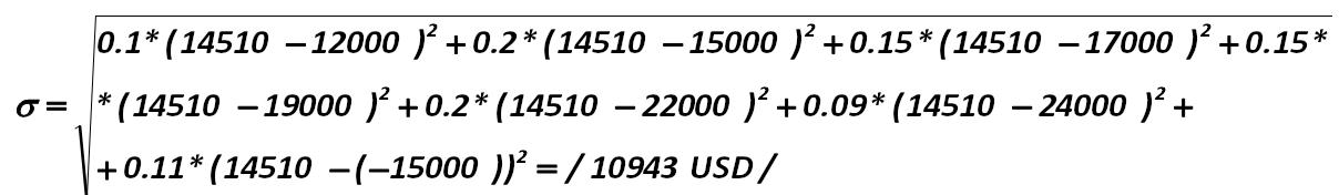
In this example, the risk for the company not to make a profit in each future period is most likely to be:
![In this example, the risk for the company not to make a profit in each future period is most likely to be: [Alexander Shemetev]](/img/s/shemetew_a_a/alexandershemetevthebankruptcyanalysisrecommendedinrussia/e1.jpg)
This 32,402 value shows the average probability deviation of amounts of expected revenue of this IE in the next month. That is, the IE will receive 14,510 USD of income in the next period. However, with a high probability, this quantity will vary from -1,691 to 30,711 USD of income. Such a high probabilities" oscillation of income obtaining is due to probability of obtaining a loss in the following month.
In addition to the absolute standard deviation (σ) it is sometimes used some other types of standard deviation in the analysis. The absolute deviation is intended to show the maximum probability of deviations from the average spread of the expected value of profits. However, if you want to estimate the most probable value of the deviation (rather than the total scale as it is in the calculation of (σ)), then use a standard measure of standard deviation (σS):
![However, if you want to estimate the most probable value of the deviation (rather than the total scale as it is in the calculation of (?)), then use a standard measure of standard deviation (SigmaS): [Saint-Petersburg State University of Economics and Finance, for example, L.S. Tarasevich, P.I. Grebennikov, A.I. Leussky]](/img/s/shemetew_a_a/alexandershemetevthebankruptcyanalysisrecommendedinrussia/244.jpg) (244)
(244)
Where: Ai - is the likelihood (probability) of each i-th value of the parameter X.
The above calculation corresponds to the weighted approach to analysis of variance. For example, a standard measure of standard deviation for IE "N.I. Stella" will be the value:
This quantity represents the total probability no longer; this quantity represents the most probable scatter of level of income for the IE "N.I. Stella": + / - 5471 USD from the magnitude of the average expected return.
However, along with the variation approach, there is an information-atomic approach [14], which also consists of the classical and the weighted sub-approaches. This approach is based on the theory of avoiding excessive mathematical information, and it carries the index of n1 observation. The theory is in just getting rid of it, turning it to the (n-1) index, knowing that it doesn"t carry any information load, due to the fact it can be easily calculated from the algorithm itself.
Atomicity of the approach is that it calculates the fair value of the deviation for a single atomic ("indivisible," "independent") element rather than the same value for the total sample.
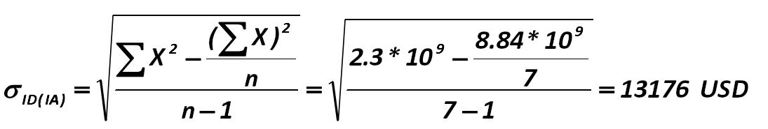
The classical school of information-atomic approach involves the following calculation of the absolute standard deviation:
![The classical school of information-atomic approach involves the following calculation of the absolute standard deviation: [Prominent advocates of this approach to the analysis are the John E. Hanke, Artur G. Reitsch, Dean W. Wichern, V.P. Nosco (Moscow State University), K. Dougerti, A. Aivazian, V. Mkhitaryan and others.]](/img/s/shemetew_a_a/alexandershemetevthebankruptcyanalysisrecommendedinrussia/245.jpg) (245)
(245)
So, for our IE "Stella" the value of standard deviation is:
(233)
(234)
(235)
(235.1)
(236)
month-aver
- this is the average value of liabilities to be paid. It can be calculated for a going-concern as the amount of short-term borrowed funds (STL) for the reporting period to a number of months in that period. Revmonth-aver
- this is the average value of revenue. It can be calculated similarly to indicator AvLmonth-aver
, and instead of STL one should use the proceeds (Rev). (237)
(238)
(239)
The debt must be less than 100,000 [7] rubles (circa it is more than 3,000 USD).
For individual entrepreneurs (IE) this amount is reduced to 10,000 rubles.
Penalties, sanctions" sums, arrears of wages and penalties are not included in the principal amount of debt.
There must be three months of overdue of debt.
There must be an entered-into-legal-force court decision on recovery of the debt or a decision of the tax authority or the decision of the customs authority.
Only a legal entity (no individuals) may file for bankruptcy.
(240)
(241)
- this is the average value of observed variables X and Y; Cov (X, Y) - is a ratio of covariance, which shows the relationship between two variables; (242)
(243)
- the average value of X, calculated by the formula (241); Xi - the value of i-th parameter.
(244)
(245)